Fed Operations Should Be Investigated

Federal Reserve monetary policy has enormous effects on the behavior of the business cycle. These business-cycle effects, in turn, affect the political environment. For example, the surge in consumer price inflation in 2021-22 appeared to be an important factor in the 2024 presidential election. In previous commentaries, I have argued that Fed monetary policy in 2020-21 exacerbated the inflationary environment in 2021-23. In my July 8, 2025 commentary “Fed Operating Behavior – Don’t Let the Perfect Be the Enemy of the Good”, I argued that the Fed should act so as to have the sum of the monetary base plus loans and securities on the books of depository institutions (thin-air credit) grow at a constant annual rate of 5 percent. Would the business cycle be eliminated under these circumstances? No. Would the amplitude of business cycles be damped? Yes. Could the Fed legitimately be criticized for political bias if it maintained thin-air credit growth at 5% per annum, regardless of what political party held the presidency? No. Would the Fed lose its mystique? Yes.

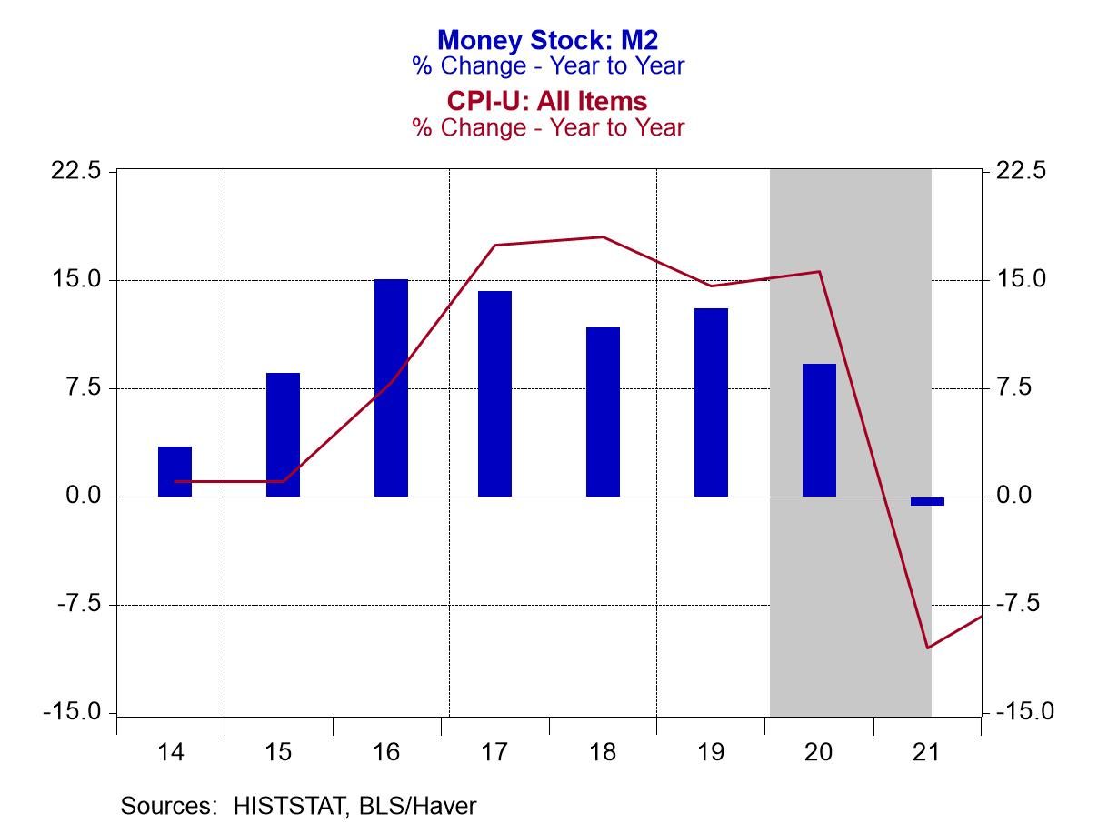
Let’s take a trip down memory lane to see how Fed monetary policy has exacerbated the business cycle. The Fed opened its doors for business in 1914, the same year that World War I started. Although the US did not enter WWI until April 1917, we were supplying war materiel and foodstuffs to the Allies prior to our entry. Plotted in Chart 1 are the year-over-year percent changes in the annual average M2 money supply (annual data for thin-air credit did not become available until 1946) and the annual average CPI. Growth in the M2 money supply accelerated to 8.5% in 1915 from 3.4% in 1914. In the six years ended 1920, M2 grew at a compound annual rate of 11.9%. And you know what else grew rapidly in these six years? The CPI. In the six years ended 1920, the CPI grew at a compound annual rate of 12.2%. So, right out of the box, the Fed was aiding and abetting consumer price inflation.

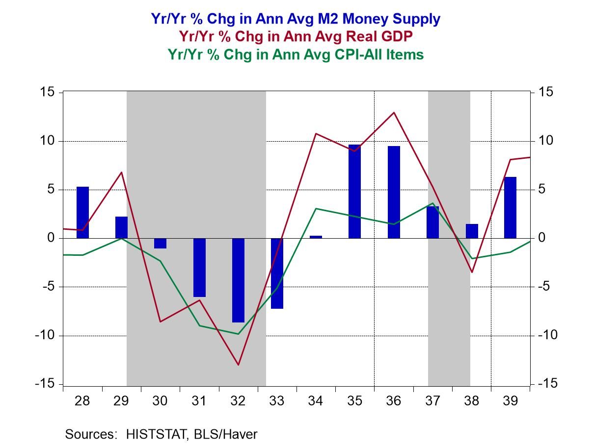
Let’s fast forward to 1928. As shown in Chart 2, in 1929, annual growth in M2 slowed to 2.2% from 5.3% in 1928. Recall that the US stock market crashed in October 1929. Did the Fed maintain M2 growth even at 2.2% in 1930? No, M2 contracted in 1930, 1931, 1932, 1993 and grew at only 0.2% in 1934. Had the Fed maintained M2 growth even at only 2.2% starting in the early 1930s, the severity in the contraction in real GDP and the deflation would have been mitigated. Then the Fed allowed M2 to grow at 9.6% and 9.5% in 1935 and 1936, respectively. Fearing that price inflation would take flight, the Fed took actions in 1937 that resulted in the sharp slowing in M2 in 1937 and 1938, which ushered in the recession of 1937. If only the Fed had maintained a steady rate of growth of 5% in M2 from 1929 through 1938 one could legitimately speculate that the severity and length of the recession that started in 1929 would have been less and shorter and that there would not have been a recession starting in 1937. There were political ramifications from the Fed’s misguided monetary policy starting in 1929. Namely, the election of FDR in 1932 and his New Deal policies that resulted in unprecedented federal government intrusion in the private sector of the economy. Although some of these New Deal policies might have been called for at the time of the deep and prolonged recession of 1929 through early 1933, would they have been necessary had the Fed maintained a steady rate of growth in M2 of 5%? I think not.

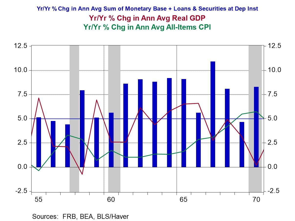
Now let’s look at the 1955 through 1970 period. Plotted in Chart 3 are the year-over-year percent changes in annual average thin-air credit rather than M2. From 1955 through 1960, thin-air credit growth was close to 5%, plus or minus, as indicated by the horizontal line in the chart at the 5% level. 5% is my back-of-the envelope rate at which I think thin-air credit should grow. The economy did incur recessions in 1958 and 1960. But these recessions were relatively mild and short-lived. CPI inflation was relatively low.

Then in 1961, thin-air credit steadily started growing faster. Starting in 1965, the CPI inflation rate started moving higher. The recession of 1970 was relatively mild and short-lived. But the CPI inflation rate had moved up to 5.7%, the highest in the 1955-1970 period.

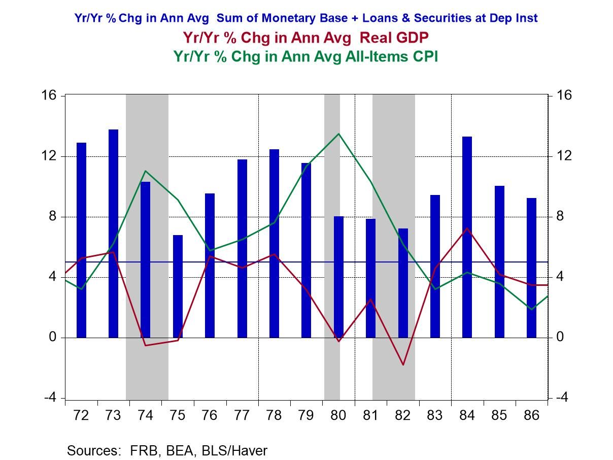
The 1971-1986 period is covered in Chart 4. From 1971 through 1973, annual thin-air credit growth soared in the range of 12% to 13.7%. In 1972 and 1973 because of El Nino, the anchovies failed to show up in the coastal waters of Peru. Anchovies are converted into fishmeal, which is a food fed to poultry and pigs. This shortage of fishmeal represented a negative supply shock to the agricultural industry. The strong growth in thin-air credit stimulated nominal aggregate demand. In the face of the shortage of anchovies, agricultural prices rose. Because nominal aggregate demand was strong, non-agricultural prices could not fall sufficiently to prevent an increase in the All-Items CPI inflation rate. This is when the “core” CPI concept, All –Items excluding food and energy prices, was introduced by Fed Chairman Burns in order to rationalize his reluctance to raise the federal funds rate so as to not harm President Nixon’s re-election chances. In October 1973, OPEC cut oil production, which represented a second and larger negative supply shock to the global economy. Even though annual thin-air growth slowed in 1974, it still came in at a hefty 10.3%. Energy prices soared, but because of relatively rapid thin-air credit growth, non-energy prices did not fall sufficiently to offset the higher energy prices. Thus, All-Items CPI inflation soared.

Thin-air credit growth took off again in the 1976-1979 period. The Iranian revolution, which began in 1978, resulted in another sharp decline in global oil output in 1979. The Iran-Iraq war of 1980 exacerbated the decline in oil production. Again, in the face of rapid thin-air credit growth in prior years, the All-Items CPI inflation rate rose. I argue that had there not been such rapid thin-air credit growth in the 1970s, the negative supply shocks that occurred then would not have resulted in as high price inflation that occurred. President Carter lost his re-election bid in 1980. The high inflation did nothing to improve his chances of a victory.

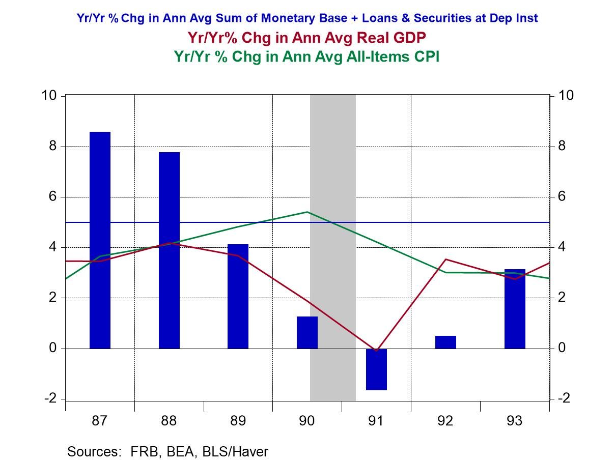
The 1987-1993 period is covered in Chart 5. The relatively rapid growth in thin-air credit in 1987 and 1988 resulted in the rise in the consumer price inflation rates in 1989 and 1990. The Savings & Loan problems that had started in 1985 brought on the creation of the Resolution Trust Corporation (RTC) to deal with failed S&Ls. The closure of depository institutions by the RTC and the FDIC in combination with the Fed’s interest-rate targeting resulted in weak thin-air credit growth in 1990-92. (The explanation of the weak thin-air credit/M2 growth during this period is laid out in a December 23, 1991 WSJ op-ed that I and unacknowledged co-author Robert D. Laurent penned, “How the Fed Subverts Its Rate Cuts”.) The resulting weak thin-air credit growth explains the recession of 1990 and the weak economic recovery of 1991. This economic weakness likely was a factor in President George H. W. Bush’s loss in his 1992 bid for a second term.

Plotted in Chart 6 are the year-over-year percent changes in annual averages of thin-air credit and the CPI. Also plotted in Chart 6 are the annual averages of household holding gains on assets as a percent of annual average Personal Disposable Income. Chart 6 covers the period from 2002 through 2008. Thin-air credit grew much above 5% in 2003 through 2006. Despite this “excess” growth in thin-air credit, consumer-price inflation was relatively low and steady. But what did move much higher was asset-price inflation (the red line in Chart 6). Prices of residential real estate and equities experienced large gains. So, in this case, excessive growth in thin-air credit was associated with inflated asset prices rather than consumer prices. (I wish some PhD student would write a thesis on explaining why excessive thin-air credit sometimes results in higher consumer-price inflation and sometimes in higher asset-price inflation.) The bursting of this asset-price bubble in 2007-08 and deep recession that followed helped Obama win the 2008 presidential election.

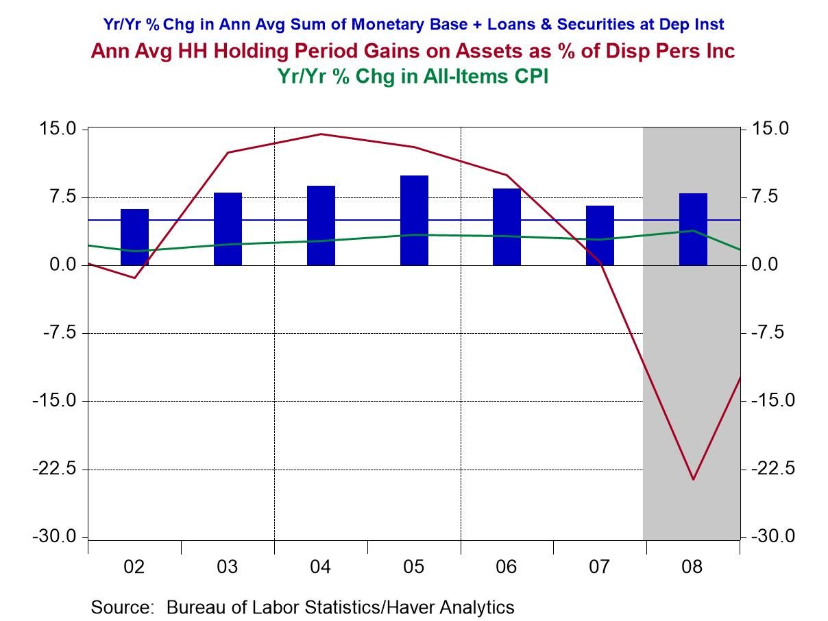
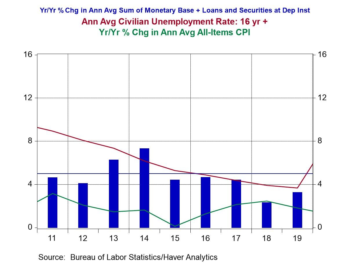
Chart 7 covers the period from 2011 through 2019. This was a period of relatively stable thin-air credit growth and thin-air credit growth close to 5% per annum. Consumer-price inflation was low and relatively steady. The unemployment rate averaged 8.9% in 2011. It trended lower over the period, reaching 3.7% in 2019. In my opinion, this was the “golden age” of Federal Reserve monetary policy, which was under the stewardship of Bernanke, who was succeeded by Yellen in February 2014, who was succeeded by Powell in February 2018. Did this relativity steady and low growth in thin-air credit during this period occur by design? Hardly. But sometimes it is better to be lucky than smart.

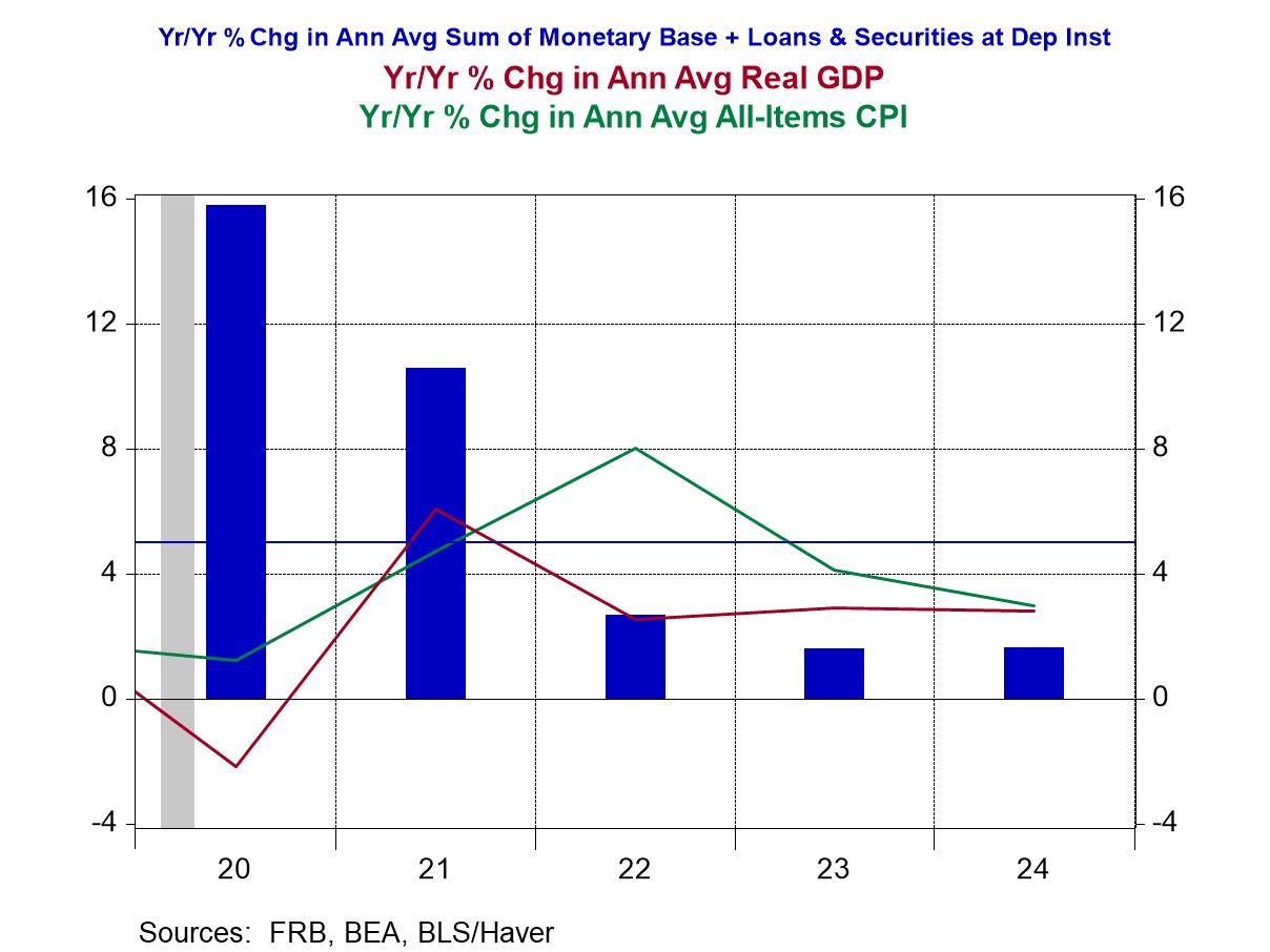
Lastly, let’s look at the period from 2020 through 2024, as shown in Chart 8. Covid hit the US in full force in March 2020. Economically speaking, Covid was a global negative supply shock. Fewer goods and services could be produced. Remember that increases in thin-air credit results in increased nominal aggregate demand. But if the real supply of goods and services cannot increase or is contracting, an increase in nominal aggregate demand will result in an increase in consumer-price inflation. Growth in thin-air credit soared to 15.8% and 10.6% in 2020 and 2021, respectively. Historically, growth in thin-air credit affects consumer-price inflation with a lag. Consumer-price inflation increased to 4.7% and 8.0% in 2021 and 2022, respectively. As I mentioned at the outset, the resulting surge in consumer-price inflation during this period following the surge in thin-air credit did Biden no favor in his 2024 re-election bid.

In summary, Federal Reserve monetary has profound effects on the behavior of the macro economy. In turn, these macroeconomic effects of Federal Reserve policy affect the political environment. Sometimes, Federal Reserve monetary policy is politically motivated. Most of the time, it is not. As Friedman said, there are long and variable lags between when a monetary policy action is taken and when its maximum impact on macroeconomic variables takes place. My research regarding growth in thin-air credit indicates that its effect on real GDP occurs within a year; on inflation, two years. But as I showed for the mid 2000s, excessive thin-air credit growth seemed to affect asset prices rather than consumer prices. How can the Federal Reserve policymakers know when their actions will affect consumer prices or asset prices? (Not until that PhD student completes his thesis on the subject.) There are data lags and data revisions that hamper policymakers’ correct decisions in real time. Then there are exogenous supply shocks, most negative, but some positive, that the policymaker cannot predict. So, yes, it is past time to do a deep dive regarding Federal Reserve monetary policy. If there were a serious investigation of Federal Reserve monetary policy conducted by serious people, I think the investigatory results would recommend that the Federal Reserve operate so as to have thin-air credit grow at a steady rate every year. The Federal Reserve would abandon interest-rate targeting. The movement of interest rates across the maturity spectrum would be determined by the demand for credit and inflationary expectations in the context of a stated steady rate of growth in thin-air credit. Perhaps this in depth study of the Federal Reserve would uncover some optimal steady rate of growth in thin-air credit above or below my suggested 5%. Perhaps it would uncover some other monetary quantity that the Fed should have increase, or even decrease, at some steady rate. Do I think that this kind of serious investigation will take place in the current political environment? No! More’s the pity.

Note: I suspect you are tired of reading about thin-air credit. I am tired of writing about it. So, I will hold off writing about for a while.